Using Fourier transform to detect large orders: Part 1

In the last two decades, advancements in information technology have contributed in the creation of virtual marketplaces where buyers and sellers are brought together through an electronic trading platform. Electronic trading is rapidly replacing human trading in global securities markets. Therefore, human best-execution practice has naturally evolved into automated execution algorithms.

Algorithmic execution refers to a set of computer methodologies used to determine the optimal way to parcel and execute an order. The aim of execution algorithms is to minimize price impact, execution costs and visibility while maximizing trade speed and size. In particular, they are essential when handling large orders. In fact, if a large order is simply posted to the market, it will cause a strong and adverse price impact, and since bid/ask quantity tend to decrease going further from best bid/ask quotes, that will significantly deteriorate the execution price.Source: BSIC

In order to minimize price impact and visibility, execution algorithms break large orders into smaller “child” orders and spread them over time. The two most common types of algorithms are the time weighted average price (TWAP) and the volume weighted average price (VWAP). TWAP algorithms attempt to conceal the order flow by breaking a large order into equally sized parcels, which are then sent out at equally spaced time intervals. VWAP algorithms, on the other hand, breaks the order into sized parcels, which are larger when trading volume is larger; the weights of the child orders are usually determined according to the historical volume. Higher trading volume is likely to provide larger pool of matching orders and result in faster and more cost-effective execution. Below we present the visual description of the strategies: TWAP is on the left, VWAP is on the right.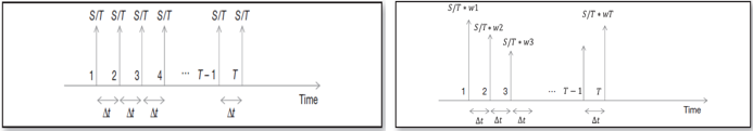Source: BSIC

From the theoretical point of view, it may be shown that using these algorithms is optimal, assuming that temporary market impact, caused by an order, decays according to power law (for reference, see Huberman and Stanzl, 2004, and Gatheral, 2009). That is a pretty realistic assumption, there are even firms specializing on estimating the function of market impact.

Those execution algorithms can really help to decrease market impact, thus optimizing the execution price. However, they present a non-negligible security flaw. Indeed, analyzing tick data, it is possible to detect the scheme, nullifying one of the main objective of the algorithm: hiding the order. The aim of our strategy consists in trying to detect and exploit hidden execution algorithms through Fourier analysis.

The procedure comprises three steps. First, we must tag all recent trades either as buy or sell; second, we have to separate those trades into bucket according to trading size and finally, within each bucket we have to identify trades occurred at identical time intervals.

The first step presents a challenge at once: in the tick data, trades are never classified as buy or sell. In fact, it is just since to every deal there are two counterparties, but we are looking for market buy/sell orders. The easiest way to classify trades is a so-called tick rule: the trade is classified with respect to the previous trade: if there is an uptick (price goes up), or zero-uptick (price stays the same, but before there was an uptick), the trade is classified as a buy, otherwise it is considered a sell. The scheme is very easy and fast in implementation, and it does not require bid/ask bounds, but its accuracy leaves much to be desired. Quote rule presents a better way of classification: the trade is considered a buy or a sell, according to which bound the trade is closer (to best offer or best bid, correspondingly). The only issue about this rule is that it cannot be used to classify trades that fall exactly at the midpoint of bid-ask spread. Indeed, we opt for the following strategy: first, we use quote rule, and then we use tick rule for the trades remained unclassified (so, we implement Lee-Ready rule; for more details, see Lee-Ready, 1991).

On the next step, we need to break our data into the bundles. Disposing the tick data provides us with a great advantage: we have all the ticks, so for us it is sufficient just to factorize the volume traded, and split our data points into the separate vectors in a way that one vector contains only data points of the same traded size.

It is the third step where Fourier analysis comes in. The key concept in Fourier analysis is Fourier transform, a mathematical construct connecting time and frequency domains. The basic idea is that complicated but periodic functions (signals) can be written as the sum of simple waves, mathematically represented by sines and cosines of different frequencies and amplitudes. The Fourier transform tells us which wave (frequency) contributes the most in defining the signal. 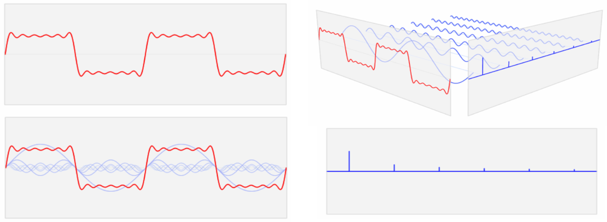Source: BSIC

or instance, it tells us that the largest blue wave is the most important in describing the red signal.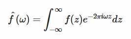

The Fourier transform for a fixed frequency w is the integral of the product between the signal f(z) (the red wave in the picture) and a complex exponential function which represents the simple sine and cosine waves (blue waves in the picture). In a sense, the Fourier transform calculates the correlation between the signal and the sine/cosine waves. In fact, the integral is an infinite sum over z and if the two functions are correlated, they will tend to be both positive or both negative for a certain z. Therefore, their product will always be positive and the value of the integral should be significant. On the other hand, if they are uncorrelated, their products will be sometimes positive and sometimes negative offsetting each other when added up and the value of the integral will be close to zero. Geometrically, the height of the bars reflects the amplitude of the waves of a given frequency, into which the initial series is decomposed.

Applying the Fourier transform to the order flow, one could detect hidden schemes buried in the noise of other trades. Let us consider another brief example. In the next picture on the left, we can see a signal obtained adding up two sine waves of frequencies 50 and 120 Hz corrupted with random noise. From the chart, it is impossible to detect any pattern in the signal but after having applied Fourier transform, we can see two clear spikes in the frequency domain in correspondence of 50 and 120 Hz. We detected the pattern through the noise.Source: BSIC

As we have shown above, the original Fourier transformation is continuous-time, so it suits perfectly for the continuous functions. Nevertheless, it cannot be used with market data, which are naturally discrete-time, so we need to implement the so-called DFT (Discrete Fourier Transform). This algorithm is powerful but very slow (it has the complexity of ). Fortunately, there exists an improved version called FFT (Fast Fourier Transform), with complexity of only . Evidently, that is a huge step up: for instance, if we consider a sample of 10⁶ observations, which is a normal quantity of daily ticks for a top-traded stock in the US (eg, AAPL), DFT will take around 20 hours to be done, while FFT will take only about half a second.

But the major drawback of all conventional discrete Fourier transformations is that they should be applied to equidistant data points (so that the time increment between two points is constant). To cope with this issue, we use the NUFFT (Non-uniform FFT), which was developed especially for non-uniform time-series.

Here is the theoretical framework of our strategy. As for the practical implementation, we have the following idea: as we have stated before, using Fourier transform, we can detect execution algorithms ex-post, but, in fact, nothing prevents us from detecting them live: if we have intraday quote stream, we can implement FFT to forecast incoming child orders. By doing this, we can benefit from the impact those orders have on the market price. Therefore, for example, if we reveal that a TWAP buy-scheme is being implemented at the moment, we may expect that it will persist for some more time, and exploit it in a simple way: buy before the expected tick, and sell after it. Since buy child orders tend to push the price upwards, this strategy may present a nice way to profit.

The backtest of this strategy, as well as the results of the application of FFT to some time-series will be presented in the next part. Do not miss the opportunity to know how HFT funds make their money.

Follow BSIC newsletter, the sequel is coming soon!

[edmc id= 3572]Download as PDF[/edmc]