Recently the spread between oil benchmark Brent and Us counterpart West Texas Intermediate has reached the highest levels in two years, breaking above $7/bbl in September. In this article we will give a brief introduction of different crude oils, the fundamental reasons behind price differentials, and an idea on how it could unfold in the near future.
Difference between WTI and Brent Crude oil
Brent Crude oil, refers to oil extracted from oil fields in the North Sea: Brent, Forties, Oseberg and Ekofisk. It is considered light and sweet, making it ideal for refining into gasoline. Brent oil due to its nature of being waterborne makes it is easier and less costly to transport to distant locations. It is used to price two thirds of the world’s internationally traded crude oil supplies.
The West Texas Intermediate is extracted from oil fields across the US and sent via pipeline to Cushing, Oklahoma where it is stored. It is sweeter and lighter crude than Brent. However, it is landlocked, meaning that it needs to rely on the capacity of pipelines and rails in order to be transported to refineries in the Gulf coast. This makes transportation more expensive. WTI continues to be the main benchmark for oil consumed in the United States.
Brent-WTI spread
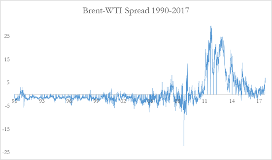
Chart 1: Brent-WTI Spread 1990-2017 (Source: EIA)
Prior to 2011, the spread between two benchmarks traded at $2-$3 premium in favour of the WTI. There was a greater supply of Brent crude as as the production in US, i.e. the WTI, was relatively low. In addition, Brent having a higher sulfur content was more expensive to refine into gasoline.
In December 2010, the Arab Spring, a series of anti-government protests, uprisings and armed rebellions spread across the Middle East. Moreover, a civil war started in Libya and escalated in February 2011. These events created concern and worries about the instability in these regions. It caused volatility in the oil market and the price of the Brent crude rallied relative to WTI crude, reason being the concerns on the availability of supplies and logistical considerations, e.g. possible violence on seaway passages. At the same time, US oil production started to rump up and determined a weakness in the WTI. For these reasons, Brent crude traded at all time high premium of $27,7 per barrel relative to WTI. Later, in 2015, the US government removed the ban for crude export, allowing companies to export crude for the first time since 1975. In combination of the proliferation of pipeline capacity, that made the transportation of crude less costly, the spread between the two benchmarks started to narrow.
Over the past 18 months, the spread has traded in a relatively restricted range of about $2-$3 a barrel. In last month though, it escalated reaching a maximum level of $7.11 due to Hurricane Harvey. The natural event created distortion in the crude oil market; it initially affected a third of US oil refineries forcing them to stop operations. This caused a temporary surge in Gasoline price and a decline in WTI, that quickly adjusted when refineries restarted operations. On 12 September WTI rose above $50 and Brent crude hit the highest level since April.
Up to now, we discussed the situation only in US and Middle East, that together with Russia represent the global supply of crude. To get a deeper insight we shall look into a huge Eastern market that cannot be ignored by any investor interested in commodities: China. This highly industrial country has been the key driver of commodities demand for the last decade and its decline in growth rate from a double digit to a “mere” 6% has brought down industrial commodities prices like copper, nickel, lead, zinc, aluminum and so on. Recently though, this commodity-behemoth has started stockpiling commodities once again, including Brent crude. Why? For the upcoming party Congress in October, an opportunity for President Xi to unveil its latest economic program of stable growth. Many expects a strategy in preparation of the not-impossible armed conflict between North Korea and the United States, either in terms of joining sides or for eventual disruption of raw material shipping lanes.
Trade Idea
Let’s now look into a trade opportunity in the market. There are mainly two questions that must be answered:
- Is China’s buying spree going to affect only Brent crude or also WTI?
- What is the current standard of Brent-WTI spread?
To answer the first question, we must recall the fundamental distinctions of crude oils: Brent is indeed the most used benchmark for pricing as two-thirds of the world employs it, including the Middle East. But computing a simple correlation analysis on Brent and WTI it is seen that correlation is around 0.93, meaning that companies consider them substitutes. Definitely there are differences in grade, transportation cost and usability, but generally they tend to move in the same way and spikes of high spreads are rare.

Chart 2: Brent-WTI Spread 2015-2017 (Source: EIA)
The second question can be answered only if we define a correct estimation window, i.e. the time-frame that we consider for “current standard”. We suggest to consider the last breaking news in the crude oil market as setting the new standard, i.e. the US opening crude oil exportation on Dec 2015. At this point, we can look into the graph and notice that generally the spread has been low on $2-$3 or even negative.
Thus, we suggest to take a long position in WTI futures and short in Brent futures to trade the reduction of the spread. One then might wonder: what time-frame? Hard to say, definitely short-term: 1-2 months or even less. The standard of $2-$3 dollars will definitely last for many more months or years, but the current level of $6 is not unseen in history and either it reverts it back in the short term or a deeper fundamental analysis must be performed.
Econometric analysis of the spread
In order to make an educated guess about the expected future value of the spread, we check what time series model best fits its past behavior. We consider the daily prices starting from 4th Jan 2016 (after Dec 2015 for the reasons stated before) to 15th Sept 2017. First of all, we perform the Augmented Dickey-Fuller Test on the Brent, the WTI and the spread: the prices of the single commodities are not stationary (the p-values of the ADF test are 83% and 80% for Brent and WTI), but we can reject the null hypothesis of a unit root in the spread with a confidence of 5%.
One of the simplest time series model is the ARMA, in which the value at time t depends on past lags of the variable itself and on past lags of the error term. The autocorrelation and partial autocorrelation function of the spread are shown in Chart 3
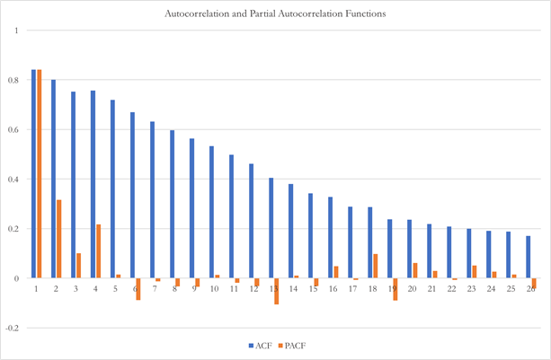
Chart 3: autocorrelation and partial autocorrelation functions of the spread (Source: BSIC)
High and decreasing values of the ACF even at remote lags, together with significant values of the PACF for the fist lags, suggest that the spread is an ARMA(2,0) or ARMA(4,0). After estimating the parameters, we discard the ARMA(2,0) model because its residuals show significant autocorrelation (a sign that we miss important information in lags after the second).
The coefficients and their p-values of the ARMA(4,0) model are shown in Table 1
| Estimate | Standard error | p-value | |
| ar1 | 0.480 | 0.046 | < 2e-16 |
| ar2 | 0.205 | 0.052 | 0.01% |
| ar3 | 0.004 | 0.052 | 94.15% |
| ar4 | 0.268 | 0.047 | 0.00% |
| intercept | 1.411 | 0.754 | 6.14% |
| sigma | 0.5256 |
Table 1: ARMA(4,0) coefficients
The deviation of the present spread level (5.73$) from the long-run expected value is 4.32$ or 2.38 times the unconditional volatility. With these parameters, we can calculate iteratively the expected spread one day ahead and the confidence interval of this prediction (here at 75%). As you can see from Chart 4, the spread is mean reverting and quickly converges to the long-run unconditional expected value of 1.41$. We set the target price of our operation at the midpoint between the current spread and the long-run expected spread, at 3.57$. The spread is forecasted to cross this level on 1st Nov 2017.
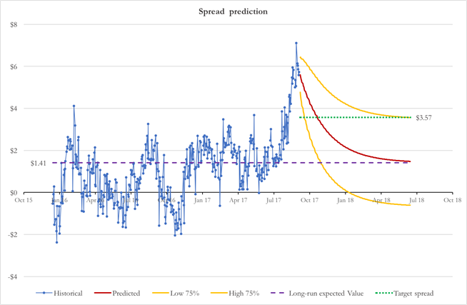
Chart 4: forecasted spread evolution (Source: BSIC)
So this is the strategy suggested by the econometrics: target spread at 3.57$ with investment horizon of 33 working days.
Implementation
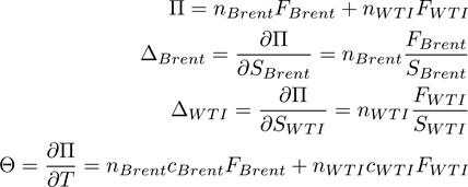
Let’s look at some practical implications: if we look at market quotes for Brent and WTI Futures on CME we notice that Brent is decreasing over time and WTI increasing over time, reducing the spread. What does it mean? From the consumption asset pricing formula
![]()
where defines a storage cost proportional to the asset value and the convenience yield. The latter represent the market ‘s expectation concerning the future availability of the commodity; the greater the possibility of shortages, the higher the convenience yield.

Chart 5: Market quotes for Brent and WTI Futures (Source: CME)
This means that the market is expecting shortages for Brent and production increase in WTI. This is line with the macro analysis of OPEC production cut, reducing supply of Brent, and fracking share oil, increasing supply of WTI. At this point it is important to ask ourselves: is it even worth trading the spread as the market is already pricing it? Our view is yes: the market is pricing inventory differentials over longer-term than us. and therefore we suggest to long WTI and short Brent on Futures on Nov-17, and if the trade wants to be continued to reroll the positions over 1-2 months in the future.
A simplified linear model
Even though there are multiple factors determining the price of futures contracts on commodities, a linear approximation can be useful to sketch a basic investment strategy. We assume that the interest rates, the storage cost and the convenience yield do not depend on the time to delivery but are characteristic to each contract and the spot price is uncorrelated with respect to the interest rate. Thus, the two future contracts are priced as follows
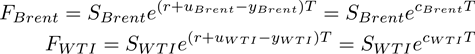
where F is the future price, S the spot price and T it the time to delivery. Our portfolio will be composed of nBrent futures contracts on Brent and nWTI contracts on WTI. As the two futures are based on different underlings, we can calculate two different measures of sensitivity to changes in the underlying, called Delta. The portfolio is also dependent on changes in time to delivery (the passage of time as the expiration date approaches), whose sensibility is measured by the Theta. In formulas
Our objective is to trade the difference between the two spot prices. To do so, we impose that the ratio of the two Deltas is equal to -1, so that the change in spot price is transmitted with the same magnitude and inverse sign to the portfolio. So, we can express nBrent as a function of nWTI. In our case we are long the WTI (nWTI>0) and short the Brent (nBrent<0) to profit from a decrease in the spread. Substituting nBrent with the formula found above, the first order differential of the portfolio is dependent only on the change in spread and passing of time.
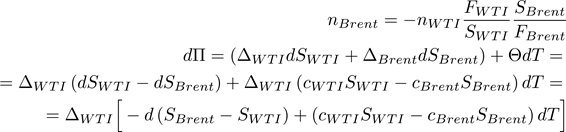
The Delta with respect to the WTI is just a constant term of scale which represent the size of our portfolio. The first term in the squared parenthesis is the negative of the change in spread. As we expect the spread to decrease, the expected effect of this term is to increase the portfolio value. The sign of the second term is undefined a priori as it is determined by the term structure of the future markets. In our case, because we are long in the WTI (in contango, cWTI > 0) and short in the Brent (in backwardation, cBrent<0), the coefficient is positive. Thus the passing of time erodes our position, other thing being equal (as time passes, the time to delivery decreases dT<0).
Our strategy is profitable as long as the expected random contribution from the mean-reverting spread offsets the time decay of the position. Using the closing prices on the 14th Sept 17 for contracts expiring at different maturities we can build different portfolios (assuming for simplicity nWTI = 1) and calculate their sensibility with respect to the spread and time to delivery.
We can use the target spread and the investment horizon which we forecasted with the ARMA(4,0) model to calculate an approximate return of the investment (Table 2). As the delivery of the contracts increase, the Deltas increase while the Theta decreases. All other thing equal, this suggest that using futures with longer maturities might increase the profitability of this strategy. However, there are other downsides with longer maturities. The first is that the portfolio is more sensible to changes in interest rate, storage cost and the convenience yield for longer times to delivery. Because the future contracts are based on a consumption assets rather than an investment assets, the time evolution on the convenience yield is determinant on the profitable outcome of the strategy, as already stated above. Last, the Deltas and Theta themselves changes with time, so the ideal strategy would be to continuously rebalance the portfolio to adjust for the changes in market prices and conditions.
| WTI | ||||||
| Month | December 17 | February 18 | March 18 | April 18 | May 18 | June 18 |
| F | $50.66 | $51.06 | $51.17 | $51.23 | $51.26 | $51.27 |
| c | 8.23% | 6.47% | 5.81% | 5.08% | 4.47% | 3.94% |
| n | 1 | 1 | 1 | 1 | 1 | 1 |
| Brent | ||||||
| Month | December 17 | February 18 | March 18 | April 18 | May 18 | June 18 |
| F | $55.22 | $55.04 | $55.03 | $55.02 | $55.01 | $55.00 |
| c | -3.88% | -2.93% | -2.45% | -2.08% | -1.82% | -1.62% |
| n | -1.023 | -1.034 | -1.037 | -1.038 | -1.039 | -1.039 |
| Portfolio | ||||||
| Initial Value | -$5.818 | -$5.864 | -$5.877 | -$5.884 | -$5.887 | -$5.888 |
| Delta WTI | 101.54% | 102.35% | 102.57% | 102.69% | 102.75% | 102.77% |
| Delta Brent | -101.54% | -102.35% | -102.57% | -102.69% | -102.75% | -102.77% |
| Theta | 635.94% | 496.84% | 436.74% | 378.63% | 333.39% | 294.89% |
| cWTISWTI-cBrentSBrent | 6.263 | 4.855 | 4.258 | 3.687 | 3.245 | 2.870 |
| Expected time decay | -$0.830 | -$0.649 | -$0.570 | -$0.494 | -$0.435 | -$0.385 |
| Expected gain from spread | $2.193 | $2.211 | $2.215 | $2.218 | $2.219 | $2.220 |
| Total expected change | $1.363 | $1.562 | $1.645 | $1.724 | $1.784 | $1.835 |
| dT | 0.1306 | |||||
| d spread | -$2.16 | |||||
Table 2: portfolios built on market prices (source: Reuters)
Even if it does not consider the whole set of factors and determinants in the oil and the commodity derivatives markets, this model has the properties required to be valuably implemented and it offers a valid and robust foundation for more sophisticated investment strategies.
- Remember to close your positions prior to expiration, you definitely do not want to be liable for thousands of barrels of Oil delivery.


0 Comments