Trading the Dispersion: chapter III
Here is the final part of our series about the strategy known as dispersion trading. The article will first focus on an additional dispersion indicator we will employ to time the entry and exit points of our strategy. Then, we will derive the optimal number of portfolios of options for each underlying and each expiry to use (remember that we are using portfolios of OTM puts and calls to replicate a variance swap). Finally, we will present the result of our strategy.
A new Dispersion Indicator to time the strategy
We used a new indicator in addition to the one we mentioned in the previous articles. The dispersion indicator we mentioned before was:
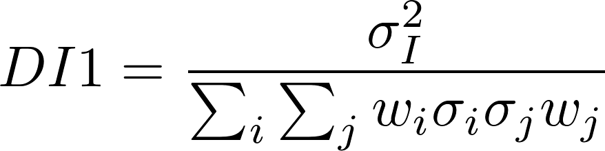
which is the 30-day index implied volatility, divided by the 30-day implied volatility of the portfolio of index constituents with perfectly positive pair-wise correlations.
The new indicator factors in the historical realized correlation between the stock and the index, giving us a better reference theoretic volatility to compare to the actual implied volatility of the index. For this, we first calculate a theoretical Markowitz implied volatility (called MIV):

(Refer to ‘Dispersion trading: Empirical evidence from U.S. options markets (2009)’ by Cara M. Marshall for derivation of the formula) Here, wi is the weight of the i-th component in the index, σi its implied volatility, ρI,i the correlation between the i-th stock and the index, hence taking into consideration only systematic risk and ridding us of the hassle of computing pair-wise correlation between all the stocks. The correlation is approximated by an historical realized correlation, calculated using daily returns and exponential weighting. The second dispersion indicator is then calculated as:
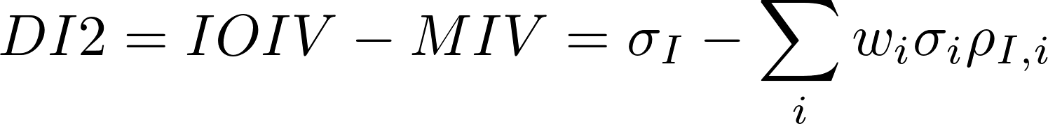
Chart 1 and 2 show DI1 and DI2 we calculated on the S&P 100. As you can see, they both shows a mean reverting behavior.
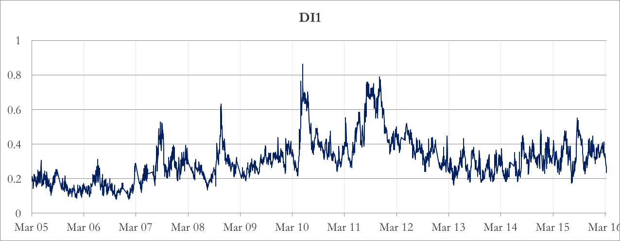
Chart 1: DI1
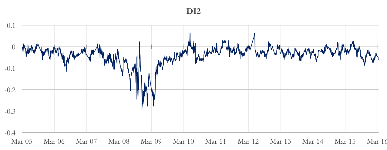
Chart 2: DI2
To determine the entry and exit point of our rategy, we use a Bollinger band approach. We calculate the historical rolling average and standard deviation of both indicators and find their z-score. If the z-score of DI1 is above 2 (below -2), we are long (short) the strategy – that is, we short (long) the 30-day index IV and long (short) the 30-day IV of the basket of components. We then square off the trade when the z-score falls (rises) to 1 (-1). As regards DI2, we enter a long (short) position using different threshold at 1 (-1) z-score due to its different behavior.
The stop-loss for a trade is based on an approach the caps the maximum loss per trade, as opposed to setting a stop loss based on the z-score. We exit a losing trade as soon as the daily loss hits 20%. The reason of such a low stop loss is to prevent the loss from few extreme returns, while not altering upward the overall P&L (at this stage, we do not want the strategy to be profitable only due to the stop loss).
In Chart 3 and 4 the z-scores of DI1 and DI2 are plotted, together with the position suggested by their values.
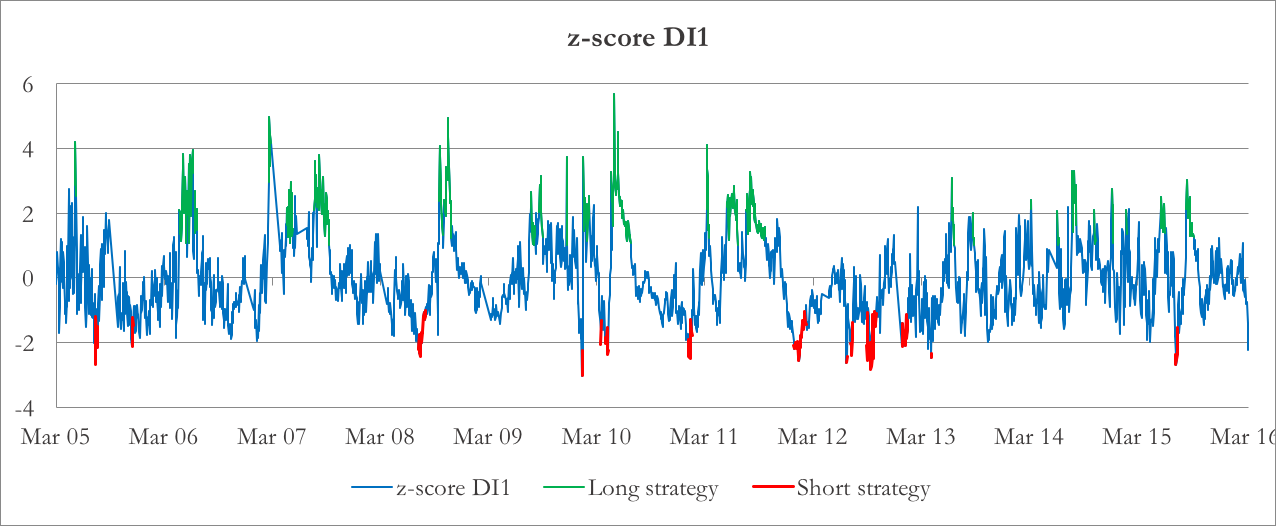
Chart 3: z-score of DI1
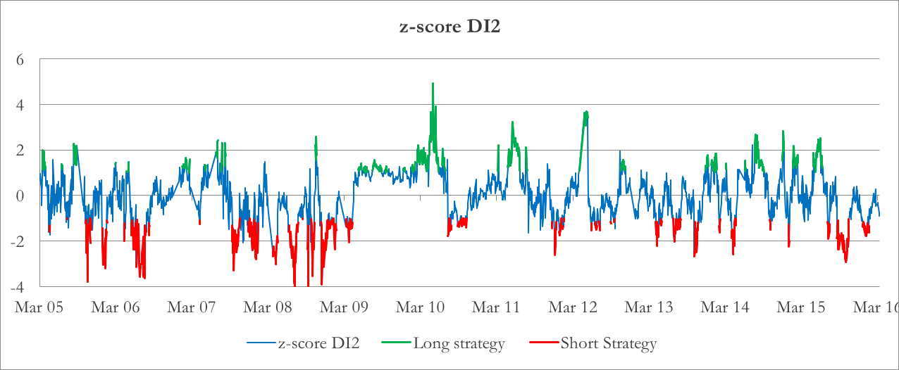
Chart 4: z-score of DI2
Targeting the 30-day Implied Volatility
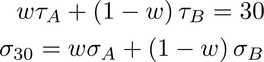
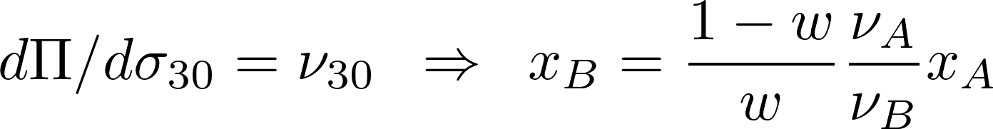
To calculate DI1 and DI2, we use a “constant time-to-expiry” 30-day implied volatility, which is obtained by linearly interpolating the implied volatility curve. In particular, it is calculated from the implied volatilities of ATM options with time-to-expiry closest but smaller and bigger than 30 days. In formula, given two options A and B, with time-to-expiry τ and implied volatility σ, we can derive the value of w from the first equation and, thus, use it to calculate the value of σ30.
Because we base our strategy on this “synthetic” implied volatility, we use options with the same expiry as A (with time-to-expiry smaller than 30) and B (with time-to-expiry greater than 30) to implement our strategy. We want our portfolio of A and B to be exposed in a predictable way to σ30, whatever change in the implied volatility surface originated the change in the 30-day implied volatility. Given the vegas of A and B νA νB (which are the sensibilities of A and B to σA and σB respectively) and the number of options xA and xB, the change in portfolio value for a small change in the implied volatility curve is approximated by a first order differential. The change in σ30 can be expressed as a differential as well.
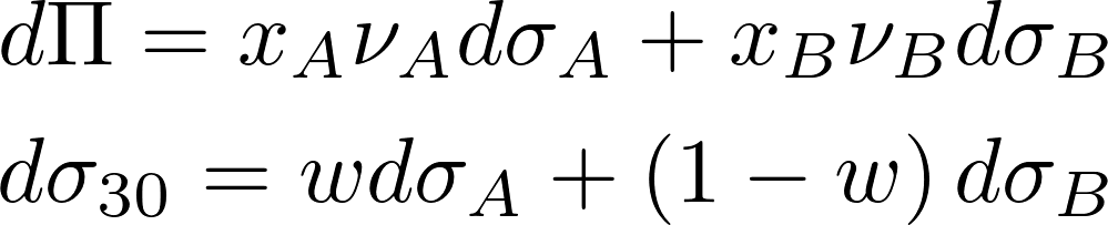
We proceed imposing that the ratio between the two differentials is constant, whatever the combination of dσA and dσB. This constant is the 30-day vega, the exposure of our portfolio to changes in 30-day implied volatility. This restriction provides a relationship between the number of options A and B.
We take into account this relationship when we mix together the two expiries. As w depends on the time to expiry of the two options, it changes as time passes, so the strategy as to be rebalanced daily to be optimal. We repeat the calculation for each underlying, then we aggregate the options on the index’s components: in this way, we have two macro-portfolios, one composed by options on the index, one composed by options on the components.
You’ve got to compromise with the weighting scheme
As already stated in the previous chapters of this trilogy, the trader that wants to build a dispersion strategy has to choose between different weighting schemes when deciding the quantities of Index options and Components options making up his portfolio.
There is no perfect solution. Pros and cons will follow whatever choice he makes. Let’s be more precise. There are 2 very well know weighting schemes: Vega-hedging and Theta-hedging. Suppose that the dispersion-trader opts for the former, then the he will build his dispersion such that the vega of the index equals the sum of the vegas of the constituents. Great! His portfolio will be immunized against short moves in the volatility. However, there is a catch. Focusing just on vega, forgetting about theta may lead to the strategy – which in principle is profitable – losing money just for the passing of time (i.e. the effect of a negative theta).
On the other hand, if the trader decides to weight components and index options such that he is Theta hedged, then he will end up with both a short vega as well as a short gamma position. As a consequence, issues may arise on the vega side and the dispersion trade ends up being not a pure bet on the dispersion.
Given all the above, a trader might decide to make a compromise. Again, different compromises could be chosen. One possibility could be that of choosing the weights in a way that the sum of the relative difference squared between the index and the components in vega and theta is minimized. This is exactly what we decided to do in our empirical application of the dispersion trade to the S&P100.
The profits
Here are the final returns of the strategy. Charts 5 and 6 show the logarithm of the cumulated return of the strategy using DI1 or DI2 as enter and exit points.
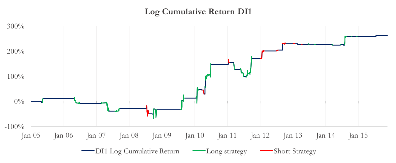
Chart 5: Logarithm of the cumulative return, using DI1
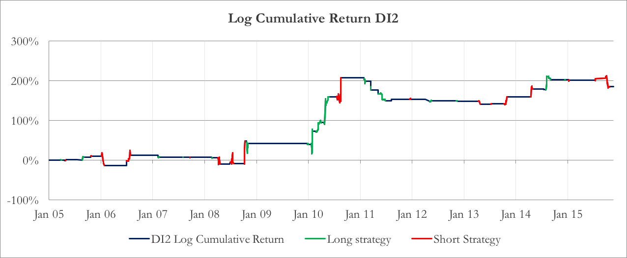
Chart 6: Logarithm of the cumulative return of the strategy, using DI2
Although the P&Ls of the two strategies look different, there are some common traits. First of all, there are few profit opportunities before 2009 for both of them, and they decrease after 2012/2013. The best year is 2010 for both: if we compare it with charts 1 and 2, you can see that in 2010 there was a substantial increase of dispersion compared to the previous year low. In Table 1 the annualized mean returns for each year are compared in detail, together with the index returns.
| Table 1 | DI1 Mean | DI2 Mean | Index Mean |
| 2005 | 10.5% | 28.5% | -0.1% |
| 2006 | -18.6% | 21.6% | 15.2% |
| 2007 | -14.7% | 58.9% | 5.3% |
| 2008 | 9.0% | 52.5% | -40.2% |
| 2009 | 58.7% | 60.8% | 22.9% |
| 2010 | 197.5% | 262.2% | 10.1% |
| 2011 | 38.6% | -49.7% | 3.8% |
| 2012 | 68.7% | 77.0% | 11.2% |
| 2013 | -2.5% | -12.7% | 26.0% |
| 2014 | 34.2% | 132.8% | 11.9% |
| 2015 | 4.2% | -9.6% | 1.5% |
The DI2 outperform DI1 in almost every year, except from 2011, 2013 and 2015. Regressing DI2 against DI1, we find that the former delivers an annualized alpha of 47.8% over the whole backtest and that the two series of returns are highly correlated (linear correlation: 0.63).
Table 2 shows some additional statistics. DI2 has both a higher annualized Sharpe Ratio and annualized mean return. If compared to the S&P100 index, both strategies have positive alpha (both significant at 10%) and are low correlated with the index. This suggests that adding this strategy to a broader portfolio would increase the expected return by delivering alpha, without adding more systematic risk.
| Table 2 | DI1 | DI2 |
| N Long days | 287 | 175 |
| N Short days | 97 | 160 |
| Ann. Mean Return | 52.7% | 85.1% |
| Ann. Sharpe Ratio | 0.81 | 1.11 |
| Alpha (vs. S&P 100) | 54.9% | 90.2% |
| Index Correlation | 0.0018 | -0.1021 |


0 Comments