Assicurazioni Generali: An Option Pricing Case with NAGARCH

Assicurazioni Generali: Business Snapshot

Assicurazioni Generali SpA is an Italy-based insurance company. It is the largest Italian insurance company and the third in the world by revenues (net earned premiums of €68,507m for the most recent available FY 2015). It operates through two segments: Life (FY 2015 net earned premiums of €48,689m and EBT of €2,599m) and Non-life (FY 2015 net earned premiums of €19,818m and EBT of €1,923m). The Life segment’s product line consists of saving and protection policies, as well as the health and pension policies. Through the Non-life segment, it provides various insurance products, such as house, car and travel insurance and reinsurance policies. Additionally, it is involved in the asset management and private-banking financial services.

The Company operates through subsidiaries in 69 countries, including Italy, Germany, France, Austria, Spain and Argentina.  The company has recently been in the spotlight, following rumors that Intesa, Italy’s largest banking operator, was planning a takeover bid on the company. As of 24 February, however, Intesa announced that it was dropping its interest in Assicurazioni Generali, as it did not match their strategic goals.

Pricing an Option: Geometric Brownian Motion, Constant Volatility

Our objective is to determine the price of a European call option with Generali’s share as underlying.[1] In order to accomplish this, we have to choose a model for the time evolution of the price of the underlying. Even if our analysis is focused on Generali, we consider two models, which can be used with any other underlying whose volatility shows the same behavior.

First, we retrieve the historical series of closing prices for Generali for the last 10 years and compute the returns y_t, using the logarithmic approximation (in our case, we will use t= 1 day).

(1) 

We need two other time series. Because the stock pays a dividend which affects the evolution of the stock price, we need the dividend yield q for the same past trading days as the closing prices. Then, we need the interest rate of a risk free asset. Since we will find the price of an option expiring in 3 months, we choose to use the 3 months’ EURIBOR.

Both the dividend yield and the risk-free interest rate are expressed as continuously compounded rates, which means that if q_year and r_year are the rates commonly expressed with one year compounding, for each maturity T

(2)

The first model we will use is a Geometric Brownian Motion with constant parameters. The equation regulating the evolution of the price is the following:

(3) 

where y_t is the return as defined in (1),  is the constant expected return,  is the volatility and e_t is a random variable with standard normal distribution.

In this approximation, volatility is assumed to be constant throughout the life of the option. This is the model at the base of the Black-Scholes-Merton equation. We take advantage of this fact to compare the implied volatility, which we derive from the BSM pricing formula and market prices for existing options of ATM Call options 3 months from expiry, with the annualized realized volatility of the returns. For each day t, the realized volatility s_t is computed as (we use 60 returns which corresponds to 60 trading days, from Monday to Friday, so that it matches the option expiry)

(4)  

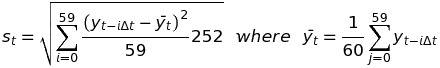
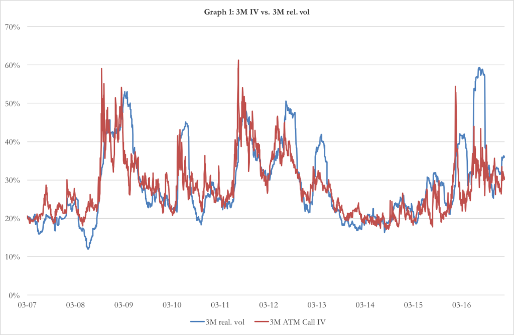
Chart 1: 3-months implied volatility vs 3-months realized volatility (source of chart data: Bloomberg)

The term 252 (which is the number of trading days in a year) is used to convert the unit of time from 1 day to 1 year. In chart 1 you can see the implied volatility and the realized volatility. There is a deep difference between the two: the former is a measure of the expected future volatility of the returns, while the latter is the measure of the past dispersion in returns. However, we can assume that the realized volatility is a good estimation of the implied volatility and use the last 3 months of past returns to calculate the constant volatility sigma of our model (3).

Following a similar approach, we estimate the constant dividend yield q with the mean of the historical dividend yield of the last 60 trading days, which corresponds to 5.13%. For the risk free interest rate r, we use the 3m EURIBOR of -0.329% (as of February 13).

Once the parameters had been estimated, we proceed to the calculation of the option price. We call a risk-neutral probability measure Q the probability measure such that the current value of a financial instrument is equal to the present value (discounted at the risk free rate) of the expected value of future cash flows.

(5) 

Under the risk-neutral probability, the expected return of every financial instrument is equal to the risk-free interest rate, so that (3) becomes

(6) 

(5) and (6) can be used together to price the European option using the Monte Carlo estimation. Monte Carlo estimation consist on 3 phases.

1- Simulate a time evolution for the underlying. Given T the time to expiry of the option, we divide the interval [0,T] into n equal intervals of length

(7)

Then we sample a series of n values z_t (with t=1 , … , n) from the standard normal distribution which are used into (6) in place of e_t to find n values for y_t.

(8)

From the series y_t we can easily calculate the price of the underlying at T S_T, given the sampled path z_t

(9)

2- Repeat the sampling and obtain the option pay-offs. We repeat the sampling from the standard normal distribution (point 1) M times and thus obtain M prices of the underlying at T, from which it is trivial to calculate M pay-offs CF_Tj of a call option with strike price K

(10)

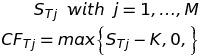
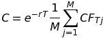
3- Take the expected value and discount. Since the evolution of the underlying followed the one under the risk-neutral probability measure, the final pay-offs CF_Tj are distributed accordingly to the risk-neutral probability measure. This means that the average of the CF_Tj is an estimator of the expected value of the option pay-off under Q. The average is then discounted to obtain the price of the call option C.

(11) 

We looked for the price of an At-The-Money call option, with S₀=K=14.77 and T=3 months. We set n=12 so that t= 1 week and iterated the sampling M=10000 times. The result is C=€0.94.

Testing the Presence of ARCH Effects

After performing the simulation with standard BS assumptions, we want to explore further possibilities that will allow us to remove some unrealistic hypothesis. The first feature that we aim to introduce in our model is time-varying volatility. A model often used for such cases is the GARCH family. In order to verify whether data show any ARCH feature, it is available a test known as Lagrange Multiplier test, introduced by Engle.  This will shed light on whether a GARCH model might be more appropriate than one with constant volatility. A standard approach for such a test is to regress our variable of interest over a constant term, and then perform the test on the residuals of such regression. However, because this test becomes more precise as the fitting of the model improves, we will first try to figure out what the best model for our data could be. We try to exploit the predictive power of a regressor, a standard one being the main stock index, FTSE-MIB, which should significantly improve fitting. The coefficient of this regression is strongly significant and this model already fits data quite well. Nevertheless, we also explore further alternatives to improve fitting even more. For instance, we try to add some autoregressive terms. We add up to 2 lags. Both lags’ coefficients are strongly significant but, because they do not improve fitting significantly, we reckon the benefit in terms of fitting is not worth the estimation of 2 parameters more. The same holds true for other lags of the FTSE-MIB. Therefore, we drop both of them. Below we show the results of our final regression:

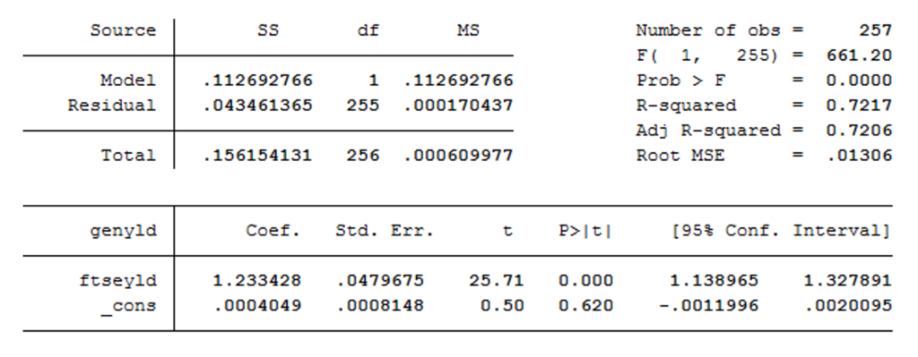Table 1: Results of regression of volatility against FTSE MIB (source of chart data: Bloomberg)

Once we have ran this regression, we can perform the LM test on residuals. The idea of the LM test is very intuitive: if we want to check the presence of ARCH effects up to , we run a regression between  and its lags up to . The test statistic is , where  is the R-squared of that regression, and it’s asymptotically distributed as a . We perform the test for lags up to 7 and our results are shown below:

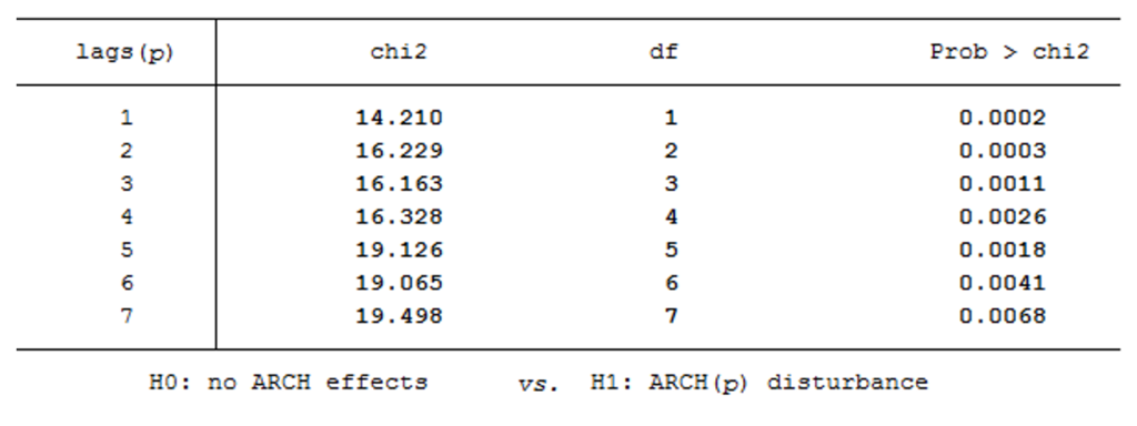Table 2: Results of test for ARCH effects (source of chart data: Bloomberg)

As we can see from p-values, we rejected the null hypothesis of no ARCH effects for each lag at a 1% significance level. However, in order to avoid parameter proliferation, we will not include all these lags in the model, but we will try to implement a model that, even if it takes account of our empirical results (as well as other features shown by financial literature), is also parsimonious.

Asymmetric Volatility: NAGARCH Model

Taken into account the fact that volatility is not constant, we want to enrich the GARCH model to take into account the fact that, in the markets, returns and volatility have negative correlation. This is a consequence of the fact that after a sharp loss of value, in particular if caused by bad news, fear makes investors anxious and volatility grows; on the other hand, after a surge in price investors become optimistic and the price stabilizes.

The model is the following:

(12) 

(13) 

Where the constants are expressed in time units of days (so that  t =1).

(12) governs the evolution of the return y. y depends on the risk-free interest rate and the dividend yield. is a risk premium term: higher the volatility, higher the risk and thus higher the expected return.  is derived when switching from difference in prices to difference in the logarithm of prices.  is a random variable with mean = 0 and variance = 1. The variance h_t of the return y_t is not constant and its evolution is given by (13). (13) is a Nonlinear Asymmetric GARCH(1,1) model. The difference between NAGARCH and GARCH is in the term , which account for the negative correlation between returns and volatility. In fact, you can derive the covariance

(14)

between the return and the variance of the subsequent period. If >0, the correlation is negative, as suggested by experimental data.

In order to estimate the parameters of the NAGARCH, we define the adjusted return y_t* which is independent from h_t and define the variable x_t as

(15)

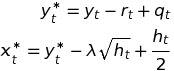
x_t is a random variable with normal distribution with zero mean and variance equal to h_t.

Given the series of x_t and a set of parameters  (where h₀ is the starting variance), we can define the log-likelihood function L as the logarithm of the product of the probability of making the observations x_t given the parameters

(16)

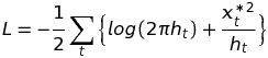
We proceed with the Maximum Likelihood Method, which consist in finding the set of parameters which maximizes the log-likelihood function. The optimization problem of maximizing L has got the following constraints:

(17)

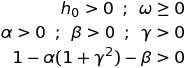
The last constraint is necessary so that the expected value of the variance is constant and positive.

In graph 2 it is showed the time evolution of the variance over last year accordingly to the NAGARCH and confronts it with the realised variance over the same period. Given that our option has a time to expiry of 3 months, we estimated the NAGARCH parameters over the last 60 days of data.

Chart 2: NAGARCH vs rolling realized variance (source of chart data: Bloomberg)

The parameters of the extrapolation are  . Under these parameters, the annualized expected volatility is 35.94%.

To check that the model is consistent with the data, we do three tests:

• Nested ARCH. We want to check if the standardised residuals  follows themselves an ARCH(1) model. The null hypothesis we do not want to reject is that the coefficients of the nested model are null, except from the constant, which is equal to 1. We find the coefficients of the nested ARCH(1) and check for their significance. They are all non-significant, except for the constant term that is different from 0 but not statistically different from 1.
• Box-Ljung Test. This test checks for the correlation of standardised residuals   series on past lags of itself. The null hypothesis we do not want to reject is that the standardised errors are independently distributed. The p-value of the test on our model is 51.34% (with lags up to 10), so we cannot reject the null hypothesis.
• Likelihood Ratio Test. We want to reject the null hypothesis that the volatility is constant. In order to do so, we consider a nested model of NAGARCH(1,1) in which each parameter is zero, except from the constant . We calculate this parameter using the Maximum Likelihood Estimation, where we call L0 the maximum value of the log-likelihood function under this restricted model and L1 the maximum value of the log-likelihood function under NAGARCH(1,1). In this case, L₁ = 146.7138 and L₀= 0141. Under the null hypothesis, the random variable

(18)

Follows a chi-squared distribution with 4 degree of freedom. The p-value of this test is 0.95%, so we can reject the constant variance model with a significance level of 1%.

After having estimated the parameters of the time evolution of the underlying, we can use the Monte Carlo method in a similar way as we used in the first case. First, we have to state (12) and (13) under the risk-free probability measure.

(19)

(20)

where

(21)

As dividend yield, we choose to use the average dividend yield of the past 3 months, while as risk free interest rate the 3m EURIBOR. Moreover, we choose =1 day, so that n=T=number of days until expiry of the option. We than proceed to sample n random variables z_t (t=1,…,n) from a standard normal distribution. As the model for the underlying has a non-constant volatility, at first the series z_t is placed in (20) at the place of e_t from t=1 to t=n in order to recursively obtain a series of n variances h_t. The variances h_t are then used in (19) with e_t to compute the series of n returns y_t.

The remaining part of the Monte Carlo method is the usual. We calculate the final price of the underlying at time T S_T as in (9). Repeat the sampling of z_t, generation of variances h_t and final price ST M times, thus having a series S_Tj (j=1,…,M) of M final prices, as in (10). From these, we calculate the pay-off of the call option with strike K. Eventually, the price of the option is the discounted value the mean of the different CF_Tj previously obtained.

In our case, we had T=61 days=3 months, r= -0.329%, q=3.97%, M=1’000’000, K=S0=14.77 (At-The-Money call). Here is the output of the Monte Carlo Method.

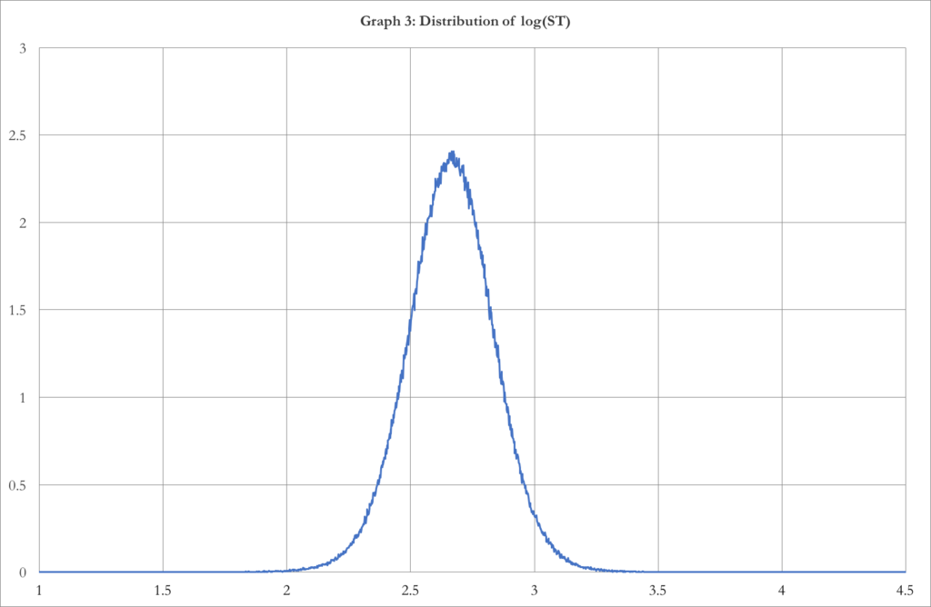
Chart 3: Distribution of log (ST) (source of chart data: Bloomberg)

Chart 3 shows the distribution of the final prices S_T. The distribution is negatively skewed by -0.08792 (which is due to the asymmetry of the NAGARCH) and has an excess kurtosis of 1.5641 (which means higher tail risk than a normal distribution, coherent with the real market distributions). We can do a Jarque-Bera test on this distribution. This test checks the null hypothesis that the skewness and the excess kurtosis of the distribution are both equal to zero. The p-value of the test is smaller than 2.2*10^-16, so we can reject the null hypothesis with any level of significance.

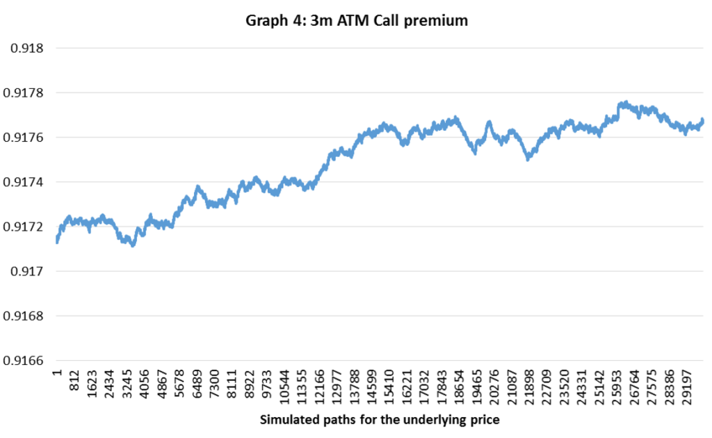
Chart 4: Simulated 3-months ATM call premiums (source of chart data: Bloomberg)

As can be seen, the price of the ATM call option converges quite rapidly to the final value C=€0.9177.[2]

One last remark, the implied volatility of the price so obtained is 35.36%, compared to the expected volatility of the NAGARCH of 36.25%.

[1] We acknowledge that American options are the standard for single names. However, we decide to proceed with the pricing of a European option for reasons of parsimony. The analysis is carried out with data up to February 13 2017.

[2] As it can be appreciated, the premium obtained with the refined NAGARCH model (€0.9177) is consistent with the premium obtained using the standard geometric Brownian motion simulation approach (€0.94).

Download as PDF